Big picture intuition for statistical inference under the random sampling framework.
Published
September 17, 2025
What is Statistical Inference?
Observational data is inherently random: if we were to measure the same variables repeatedly, we would almost certainly get different values each time. A classical explanation for the source of this randomness is the model-based (or sampling-based) perspective. In this abstraction, we assume there exists an underlying superpopulation or data generating process (DGP): a fixed but unknown probability distribution \(F\) that can, in principle, generate infinitely many observations. Randomness then arises because we only observe finitely many realizations from \(F\) — never the entire distribution. Within this framework, we define statistical inference as the process of using the observed random data to estimate features of \(F\) and quantify the uncertainty in those estimates.
Notice that the exposition above implicitly assumes that there is a single underlying distribution \(F\) from which all observed data are drawn. To make this mathematically precise, we need to introduce the random sampling assumption. This provides the framework to connect the observed data to the DGP, and thereby lays the foundation for statistical inference.
The Random Sampling Framework
The discussion going forward will primarily focus on cross-sectional datasets. These consist of several observations of a collection of variables for a given point in time and can be denoted as
Since observational data is random, it is natural to we view the observed data vector \[
\boldsymbol{x}_i = (x_{i1}, \ldots, x_{iK})' \in \mathbb{R}^K \quad \text{for } i = 1, \ldots, n,
\] as a realization of the random vector \[
\boldsymbol X_i = (X_{i1}, \ldots, X_{iK})' \in \mathbb{R}^K \quad \text{for } i = 1, \ldots, n,
\]
with some associated probability distribution. For example, we can think of the CPS dataset as consisting of random vectors
\[
\boldsymbol X_i = (sex_i, age_i, educ_i, wage_i)' \quad \text{for } i = 1, \ldots, n.
\] For some specific individual \(i\) in the CPS dataset, we then observe the vector of realized values1
\[
\boldsymbol x_i = (1, 25, 16, 25000)'.
\] Intuitively, the distinction between the random vector \(\boldsymbol X_i\) and the realization \(\boldsymbol x_i\) is that the former represents the \(i\)-th observation before viewing the data (unknown and random) and the latter represents the \(i\)-th observation after viewing the data (specific known value).
Random Sampling
We have now represented the dataset as a collection of random vectors \(\boldsymbol X_1, \ldots, \boldsymbol X_n\), each with some probability distribution \(F_1 \ldots, F_n\). However, the connection between the underlying DGP and the observed data remains unclear. Specifically, we need a simplifying assumption that will allow us to connect the distributions of each \(\boldsymbol X_i\) to the underlying DGP in a straightforward manner. The simplest framework is that of random sampling. Here, we assume that the random vectors \(\boldsymbol X_1, \ldots , \boldsymbol X_n\) are independent and identically distributed (iid) with some common but unknown distribution \(F\) on \(\mathbb{R}^K\). Thus, under this assumption, the data generating process is precisely the distribution that governs each individual random vector \(\boldsymbol X_i\).
Alternative Assumptions
The random sampling assumption is one potential way to characterize the dependence structure across the observed data points. It is popular because (i) it is often reasonable when working with cross-sectional datasets2, and (ii) it is the backbone of several statistical theorems and methods.3 However, it does not necessarily have to hold. For example, we often work with data where the units are connected via some underlying factor (location, industry, etc.). In such cases, the assumption of independence across individual units is violated. An alternative approach in such cases is to instead assume mutual independence across clusters of units. Another example of a violation to the independence assumption is time-series data, where the individual unit is indexed by time. Here, consecutive observations are usually correlated and independence is instead formulated in terms of stationarity and other concepts outside the scope of this post.
Notation and Example
The discussion so far has purely been conceptual, and so it is useful to consider a concrete example. Before doing so, however, let’s clarify some notation used in the random sampling framework. We denote the population-level random variables as \(X_1, \ldots, X_K\). The data generating process \(F\) is the joint distribution of these random variables. For example, \(X_1\) could denote the generic random variable for wage in the entire US population and we are interested in making inferences about its distribution. We denote the sample-level random variables as \(X_{i1}, \ldots, X_{iK}\). These represent the random variables associated with specific units in the sample. Continuing the example, \(X_{i1}\) denotes the random variable representing the wage of individual \(i\) in the sample. Finally, we denote the realized observations as \(X_{i1}=x_{i1}, \ldots, X_{iK}=x_{iK}\). These are the actual values we observe. So, \(X_{i1} = 25,000\) means that the observed wage of individual \(i\) is \(25,000\).
Now suppose our data generating process consists of one random variable with an exponential distribution with scale parameter \(\beta = 1\): \[
X \sim \text{Exp}(1) \quad \text{with density } f(x) = e^{-x} \text{ for } x \geq 0.
\]
If we assume our dataset is a random sample of size 30 from the above DGP, then \[
X_{i} \sim \text{Exp}(1) \, \, \text{ for } i = 1, \ldots, 30 \quad \text{and} \quad X_i \perp X_j \, \, \text{ for } i \neq j.
\]
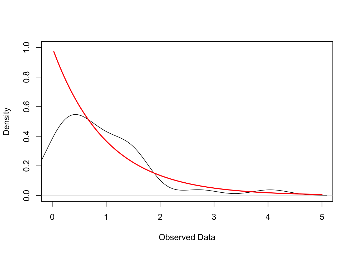
The figure below plots the empirical kernel density of such a random sample (black line) and the true density of the exponential distribution (red line). In practice, we do not know the true DGP and need to guess its characteristics using the observed data. Randomness in the finite observed data makes this a non-trivial task — as illustrated by the discrepancy between the empirical and true densities in the figure below.4
Code
# Simulate IID sample of 30 obs from exp(1)set.seed(123)n <-30x <-rexp(n, rate =1)# Empirical Density dens <-density(x)# True Exponential Densityxs <-seq(0, max(x), length.out =200)ys <-dexp(xs, rate =1)# Plotplot(dens, main ="", xlab ="Observed Data", ylab ="Density", xlim =c(0, 5), ylim =c(0, max(c(dens$y, ys))))curve(dexp(x, rate =1), from =min(x), add =TRUE, col ="red", lwd =2)
Point Estimation
Point estimation is the first step of statistical inference, and involves constructing a “good guess” for a feature of the unknown data generating process. To be more precise, this feature is called an estimand\(\theta\) and is defined as a function of the data generating process \(F\):
\[
\theta = \theta(F).
\]
An example of an estimand is the the population mean of a random variable \(X\): \[
\mu = \mathbb{E}_F[X].
\]
Since the DGP is unknown, the best we can do is use the observed data to guess the value of the estimand. An estimator\(\hat \theta\) is a function of the sample that is intended to provide a guess of the estimand:
When the estimator is evaluated at a specific realization of the sample, we obtain an estimate\(\hat\theta(\boldsymbol x_1, \ldots, \boldsymbol x_n)\) of the estimand. It’s worth emphasizing that the estimand is a fixed but unknown number, the estimator is a random variable, and the estimate is a fixed and known number.
In statistics, there are several estimation principles that provide systematic ways (i.e. rules) to construct estimators. One common method is the analog principle (or plug-in principle). The idea is to construct the estimator by replacing the population quantities in the estimand with their sample analogs.5 Thus, the analog estimator for the population mean is the sample mean, defined as
How do we know if an estimator is any good? To answer this question, statisticians study desirable properties that an estimator should ideally satisfy. A full treatment of estimator properties is typically the focus of a mathematical statistics course, but it is still valuable to briefly highlight some fundamental properties here.
The error of an estimator is defined as the difference between the estimate and the estimand:
\[
e(\boldsymbol x_1, \ldots, \boldsymbol x_n) = \hat\theta(\boldsymbol x_1, \ldots, \boldsymbol x_n) - \theta.
\] The bias of an estimator is the average error of the estimator across all possible samples of size \(n\) from the DGP:
\[
B(\hat\theta) = \mathbb{E}_F[\hat{\theta}] - \theta
\] Intuitively, the bias captures the systematic error of the estimator: if the bias is positive, the estimator tends to overestimate the estimand, and if the bias is negative, the estimator tends to underestimate the estimand. We say an estimator \(\hat{\theta}\) is unbiased for \(\theta\) if its bias is zero:6
\[
\mathbb{E}_F[\hat{\theta}] - \theta = 0.
\] Thus, the errors of an unbiased estimator are purely due to randomness in the data. As it turns out, the sample mean is an unbiased estimator of the population mean under the random sampling assumption:
\[
\mathbb{E}_F[\hat{\mu}] = \frac{1}{n} \sum_{i=1}^n \mathbb{E}_F[\boldsymbol X_i] = \frac{1}{n} \sum_{i=1}^n \mu = \mu.
\] The first equality follows from the linearity of expectations, the second equality follows from the random sampling assumption, and the third equality is a simplification.
While bias quantifies how far the estimator’s average is from the estimand, the variance (or sampling variance) measures how much the estimator varies across repeated samples of size \(n\):
\[
Var(\hat\theta) = \mathbb{E}_F[(\hat\theta - \mathbb{E}_F[\hat\theta])^2].
\] The variance of the sample mean under the random sampling assumption is given by
\[
\operatorname {Var} \left[\hat\mu\right] = \frac{1}{n^2}\operatorname{Var} \left[ \sum_{i=1}^n \boldsymbol X_i\right] = \frac{1}{n^2} \sum_{i=1}^n \operatorname{Var}[\boldsymbol X_i] = \frac{1}{n^2} \sum_{i=1}^n \sigma^2 = \frac{\sigma^2}{n},
\] where \(\sigma^2\) is the population variance \(\operatorname{Var}[X]\). The first equality uses the properties of variance. The second equality follows from the fact that the independence of each \(\boldsymbol X_i\) means they are uncorrelated, and so the variance of their sum equals the sum of their variance. The third equality uses the fact that each \(\boldsymbol X_i\) are drawn from an identical distribution and so have the same variance \(\sigma^2\). The fourth equality is an algebraic simplification.
The Necessity for Statistical Models
The sampling distribution of an estimator is the probability distribution that describes how the estimator’s estimates vary across all possible samples of size \(n\) drawn from the DGP. Intuitively, it characterizes the behavior of the estimator under repeated sampling. Under the random sampling assumption, the sampling distribution is completely determined by the DGP \(F\), the sample size \(n\), and the functional form of the estimator \(\hat\theta\).
Let’s revisit the example of the sample mean estimator \(\hat\mu\) for the population mean \(\mu\). We have already established some features of the sampling distribution of \(\hat\mu\) despite knowing nothing about \(F\). Particularly, the mean of \(\hat\mu\) is \(\mu\) and its variance is \(\sigma^2/n\). However, to say more about the distribution of \(\hat\mu\) — like its shape — we need to make assumptions about the DGP.
A statistical model is a set of assumptions about the general structure of the data generating process \(F\). Put differently, we can think of a statistical model as a family of possible distributions that \(F\) could belong to. To illustrate the added value of statistical models, suppose our sample \(\boldsymbol X_1, \ldots, \boldsymbol X_n\) is drawn iid from \(\mathcal{N}(\mu, \sigma^2)\). Since
is a linear combination of normally distributed random variables, it is also normally distributed. Moreover, we have previously established that \(\mathbb{E}_F[\hat\mu] = \mu\) and \(\operatorname{Var}[\hat\mu] = \sigma^2/n\) for any DGP \(F\). Thus, assumption of a normal DGP allows us to completely characterize the sampling distribution of \(\hat\mu\) as \(\mathcal{N}(\mu, \sigma^2/n)\). This is powerful because we can use this sampling distribution to quantify the uncertainty in our estimates by constructing confidence intervals and conducting hypothesis tests.
Constructing Confidence Intervals for \(\hat\mu\)
Conclusion
flowchart LR
  classDef box fill:#f8f9fa,stroke:#444,stroke-width:1px,rx:10,ry:10;

  DGP["Data Generating Process"]:::box
  Data["Observed Data"]:::box
  Model["Statistical Model"]:::box

  %% Main flows
  DGP -- "Random Sampling" --> Data
  DGP -. "Assumptions" .-> Model
  Model -- "Probability" --> Data
  Data -- "Inference" --> Model
  Model -. "Approximate Reality" .-> DGP
It is important to note that statistical inference is valid only if the assumptions of statistical model hold.
References
Hansen, Bruce E. 2022. Probability and Statistics for Economists. Princeton University Press.
Footnotes
Here, the value of \(1\) refers to the individual being a male and \(16\) means \(16\) years of education.↩︎
For example, if we collected data on a random subset of individuals from a large common population (e.g. the USA), it is reasonable to assume that the characteristics of one individual are independent of another individual and that they all come from the same population distribution.↩︎
Crucial theorems in asymptotic statistical theory, like the Law of Large Numbers and the Central Limit Theorem, require the random sampling assumption to hold.↩︎
Technically, under iid sampling, the empirical distribution converges to the true distribution as the sample size tends to infinity — a result known as the Glivenko–Cantelli theorem. Nevertheless, in any finite sample, uncertainty remains, and with it the need for statistical inference.↩︎
To quote my Mathematical Statistics Professor Daniel Weiner: “Do to the sample to get your estimator, as you would do to your population to get your estimand.”↩︎
To be more precise, \(\hat\theta\) is unbiased for \(\theta\) if \(\mathbb{E}[\hat\theta]=\theta\) for all \(F \in \mathcal{F}\), where \(\mathcal{F}\) is a class of distributions.↩︎